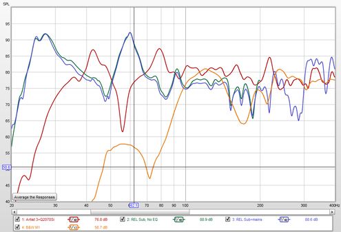
The All SPL graph is an overlay graph that shows all measurements (SPL and/or
Impedance) that have been made. It allows an average to be generated of all selected
traces or arithmetic operations to be carried out on pairs of traces to generate
a new trace.
Average The Responses calculates an rms (root mean square) average of the
SPL values of those traces which are selected when the button is pressed. That means
the dB values are converted to linear magnitudes, those magnitudes are then squared,
summed and divided by the number of measurements, the square root of the result is
taken, then the value is converted back to dB. Phase is not taken into account,
measurements are treated as incoherent. The frequency range of the averaging result
covers the region where the traces overlap, for example if one trace was measured
to 200Hz, another to 500Hz and a third to 1000Hz the average would range to 200Hz (to
the lowest end frequency). If only a single trace is selected the result has the magnitude
data from the source measurement and no phase data.
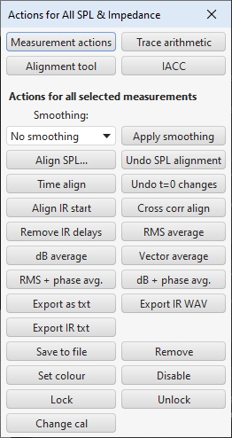
The Actions panel for the All SPL graph has these controls, there may
be more or fewer controls depending on the measurement type.

The controls are split into four groups:
- Those which apply to an individual measurement, shown by the Measurement actions button
- Trace Arithmetic controls, shown by the Trace arithmetic button
- Alignment tool controls, shown by the Alignment tool button
- IACC controls, shown by the IACC button
- Those which apply to all measurements currently selected in the graph legend
The Actions for all selected measurements are:
- A smoothing action that allows the fractional octave smoothing
setting for all the currently selected traces to be changed. The
chosen setting is applied using the Apply smoothing button
- Align SPL..., which adjusts all the currently selected SPL measurements
so that they have the same average SPL over a selected span.
- Undo SPL alignment, which reverts to the original measured level.
- Undo t=0 changes, which resets t=0 to the as measured state.
- Time align, which brings all the currently selected measurements
into time alignment. If the measurements have been made with a timing
reference (a loopback connection or an acoustic timing reference) the
impulse response is shifted according to the measurement delay value,
taking into account any IR timing offsets which have been applied
since the measurement delay was calculated. Measurements which have been
made without a timing reference are shifted according to the estimated IR
delay. Time alignment can only be applied to measurements that have an impulse
response.
- Align IR start, which aligns all the currently selected measurements
using their IR start times.
- Cross corr align, which time aligns the currently selected measurements
by cross correlation of their windowed impulse responses, using the measurement
which appears first in the list of those selected as the reference (the order of
measurements can be changed by dragging them up or down the list). This may be useful
to align measurements from a mic array or measurements of the same source from
different positions prior to vector averaging.
- Remove IR delays, which removes the estimated IR delay for all the currently
selected measurements which have an IR.
- RMS average, which calculates an rms average of the SPL values of
those traces which are selected when the button is pressed. This does the same
as the Average The Responses button, the dB values are converted to linear
magnitudes, those magnitudes are then squared, summed and divided by the number
of measurements, the square root of the result is taken, then the value is converted
back to dB. Phase is not taken into account, measurements are treated as incoherent.
If only a single trace is selected the result has the magnitude data from the source
measurement and no phase data. If the measurements were made at different positions
(spatial averaging) it is usually best to first use the Align SPL... feature
to remove overall level differences due to different source distances. When measurements
with distortion data are averaged their distortion data is also averaged, providing the
data cover the same frequency range at the same resolution.
- dB average, which averages the dB SPL values of the currently selected traces.
This produces results that are closer to what one might intuitively expect from
looking at the traces, but gives equal weight to peaks and dips which masks the magnitude
difference between them. For example, a +20 dB peak has a magnitude that is 100 times
larger than a -20 dB dip. dB averaging them produces 0 dB, 10 times smaller than the
peak and 10 times larger than the dip. dB averaging may be useful when averaging
smoothed traces to derive an EQ target, with unsmoothed data the dips would have
a disproportionate effect on the result. When measurements
with distortion data are averaged their distortion data is also averaged, providing the
data cover the same frequency range at the same resolution.
- Vector average, which averages the currently selected traces taking into
account both magnitude and phase. It can only be applied to measurements that
have an impulse response and is most appropriate for multiple measurements taken
from the same position, or measurements which have been time and level aligned
before averaging them. When measurements with distortion data are averaged using
Vector average their distortion data is also averaged, providing the measurements
were made at the same sample rate and with the same sweep settings.
- RMS + phase avg. and dB + phase avg., which produce an RMS or dB average
of the magnitudes and use vector average for the phases. They can only be applied to measurements
that have an impulse response. Both are appropriate for multiple measurements of a source.
Measurements should be time and level aligned before averaging them, cross correlation
alignment is recommended for the time alignment. These averaging methods do not exhibit
the magnitude dips due to phase cancellations that can occur with vector averaging. The
resulting impulse response may have significant acausal content as the relationship between
magnitude and phase that would normally hold is broken. As a result the average requires
larger left windows than usual. The effects of any calibration files of the individual
measurements are merged into the resulting impulse response.
- Export as txt, which exports the currently selected measurements to text files.
- Export IR WAV, which saves the impulse responses of the currently selected measurements to WAV files.
- Export IR txt, which saves the impulse responses of the currently selected measurements to text files.
- Save to file, which saves the currently selected measurements to an mdat file.
- Remove, which removes the currently selected measurements.
- Set colour, which sets all the currently selected measurements to the chosen colour.
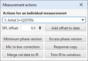
The Measurement actions dialog has the following controls:

The options for each selected measurement are to:
- Offset the measurement either temporarily or (by using
Add offset to data) permanently
- Make a Minimum phase version of the selected measurement to use in
calculations - the copy has a minimum phase impulse response and the
same magnitude response and calibration data as the original
- Make an Excess phase version of the measurement to use in
calculations - the copy is the original measurement divided by a minimum
phase version of the measurement
- Make a new measurement with Mic in box correction that has
the SPL data of the source with a correction to compensate for the
measurement being made using the microphone in box method, adding an offset
of 40*log10(f/f0) where f0 is a nominal reference frequency, which has
been set to 50 Hz. The result would usually be merged with a far field
measurement.
- Make a new measurement with Response copy that has the same
response as the measurement - the copy has the same impulse
response and calibration data as the original but does not include
distortion data or equaliser settings, for example
- Make a new measurement with Merge cal data to IR that has the same
response as the measurement but with an impulse response that includes the
effect of the measurement's cal files. There might be artefacts in the
impulse response if the cal data has large roll-offs. Note that the new
measurement will include the distortion data of the original, but the
fundamental for that distortion data will remain unchanged.
- Make a new measurement with Trim IR to windows that is a copy of the
measurement with an impulse response that is shortened to the smallest power of
2 that covers the windowed span, starting at the beginning of the left window.
This might be useful for shortening an IR before export or to shorten the IR from
an arithmetic result that produces a long IR.
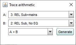
The Trace Arithmetic controls allow the chosen pair of traces to be
added, subtracted, multiplied, divided, coherently (aka vector) averaged or merged.
Either of the traces may also be inverted (magnitude, phase or both). Division and
inversion can be restricted to a frequency range with the response left unchanged outside
that range. If both the chosen traces have impulse responses,
the result will also have an impulse response, however the sample rates must be either the
same or related by an integer. For example, traces at 44.1kHz and 11.025kHz can be combined
via an arithmetic operation, the result will have the higher of the two rates. This allows
operations on band limited measurements which may have been decimated to a lower sample rate.

If the traces have incompatible sample rates, or neither has an impulse response,
the result will not have an impulse response, but it may have both magnitude and phase
data if both the traces it was applied to had magnitude and phase data, otherwise the
result will only have magnitude data and the traces will be treated as incoherent.
If one trace has an impulse response and the other does not the result will have an
impulse response. This could be used to merge a cal file response with an IR or apply
a target response adjustment to an IR.
The frequency span of the result of an arithmetic operation will be from the lowest
start frequency to the highest end frequency of the traces operated on. Outside their
frequency range traces are treated as being zero valued, with the exception of the divisor
in a division operation which is treated as being unity outside its range. If the
measurements actually have significant levels outside the measurement range the zero
setting will generate oscillations in frequency and time domains, for best results use
traces that span the full frequency range.
Trace arithmetic notes
- For meaningful results measurements that have impulse responses or phase data should
be properly time aligned before they are combined. Being properly time aligned may mean
having a common timing reference or may mean removing time delays, it depends on the
operation and what you are trying to achieve. An exception is the Merge operation,
for which REW will automatically align both magnitude and phase at the merge frequency,
adjusting the trace B time delay as required for the phase match. The amounts of the
adjustments are shown in the notes of the newly generated measurement.
- The currently applied impulse response window settings are used for each trace. The
result uses the same window settings as trace A unless the operation was Merge B to A,
in which case the window settings for trace B (the low frequency portion) are used,
or for division and inversion, which use windows that span the entire resulting impulse
response as the result is typically not causal. The
window reference time for the result will be at the peak of the result IR. The
left window width will be increased if necessary so that it is at least twice the span
from the start of the result IR to its peak to avoid truncation artefacts in the result.
Any frequency-dependent settings are excluded, applying an FDW to the result would amount
to applying the window twice, as it is already applied to the data used to produce the result.
- The result of arithmetic on measurements that have compatible impulse responses is
smoothed using the measurement A smoothing, unsmoothed data is used during the calculations.
Other measurements use whatever smoothing they already had applied during the calculations
and the result is treated as unsmoothed (or 1/48 octave smoothed if data is 96 PPO).
- The division operations have an optional regularisation parameter which is
defined as a percentage of the average level of the divisor. By default the parameter
is zero, meaning no regularisation. Applying regularisation limits the boost which occurs
when the divisor becomes very small (or zero!), such as where the divisor has notches in its response,
and so produces a more stable and manageable result. The maximum gain corresponding to the
regularisation percentage is shown next to the control, at 25% (the maximum setting) no gain
is allowed. Division may also be constrained to operate within a desired frequency span, with
an upper and/or lower frequency limit. Outside those limits inversion division reverts
to the numerator, blended over a 1 octave span centred on the limit frequency.
- The inversion operations have a maximum gain parameter which limits the boost which occurs
when the response being inverted becomes very small (or zero!), such as where there are notches,
and so produces a more stable and manageable result. Inversion may be constrained to operate
within a desired frequency span, with an upper and/or lower frequency limit. Outside those
limits inversion reverts to unity gain, blended over a 1 octave span centred on the limit
frequency. Inversion also provides a target level for the inversion to use, or a check box
to set the target automatically based on the average level of the measurement, and an option
to exclude parts of the response that look like notches from the inversion. The 1/|A| and
1/|B| operations produce a linear phase result.
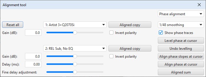
The Alignment tool allows gain, polarity and delay adjustments to be made to a
pair of measurements with a live preview of the summed result updated as the parameters are
changed (the preview uses log spaced data at 96 PPO so may differ slightly from the final
result). There is also a dotted trace which shows the result of a summation of the measurements
ignoring phase. When the alignment tool is opened the All SPL graph selections change to show
only the traces being aligned. Other traces may be selected in the graph legend if desired. The
original trace selections are restored when the alignment tool is closed.
There are two sliders for delay adjustment of the B measurement, one for coarse
adjustment and one for fine to provide a wide adjustment range. The tool can operate in phase
or impulse alignment modes.

The Aligned copy buttons generate a copy of the selected measurement with the
alignment gain, delay and polarity selections applied. Aligned sum generates
a new measurement with the summed results of the alignment settings.
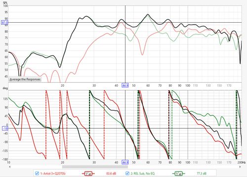
When Show phase traces is selected in phase alignment mode the All SPL graph is
split with the SPL traces at the top and phase traces for the two selected measurements and
the aligned sum at the bottom.

The Level phase at cursor button calculates the delay required to bring
the first measurement phase trace to be approximately horizontal around the frequency
of the cursor in the phase trace graph. Both measurements have the same delay applied
so the relative delays required to align them are not affected. Shifting the phase traces
in that way makes it easier to align them. The delay is only used to update the phase
traces, it is not applied when using Aligned copy or Aligned sum.
Undo levelling removes the levelling delay from both measurements.
The Align phase slopes at cursor button calculates the measurement 2
delay required to give both phase traces approximately the same slope around the
frequency of the cursor in the phase trace graph, so they have approximately the
same group delay. Note that the phase traces may still be far apart, particularly
if one measurement is out of phase with the other. In that case inverting one of
the measurements would bring the phase traces closer together.
The Align phase at cursor button calculates the measurement 2 delay
required to bring both phase traces as close as possible to each other around the
frequency of the cursor in the phase trace graph. Note that a better overall
alignment might be achieved by inverting one of the measurements and then aligning
phase, and/or by manually adjusting the delay.

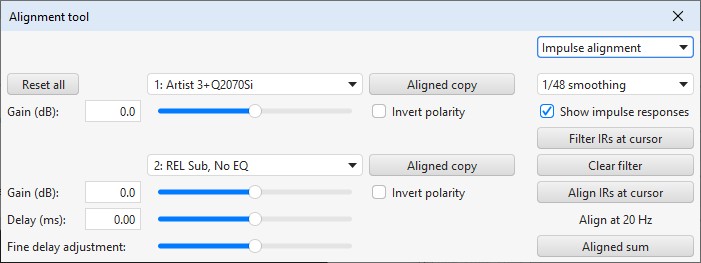
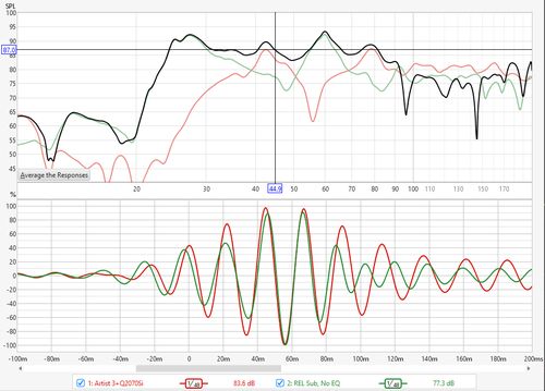
When Show impulse responses is selected in impulse alignment mode the All SPL graph is
split with the SPL traces at the top and impulse responses for the two selected measurements at the
bottom. To perform impulse alignment the responses are filtered at the cursor frequency with a 1/3
octave zero phase filter, the filtered responses are then aligned. The time span of the filtered
impulse response graph adjusts to suit the alignment frequency.

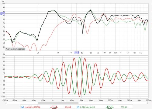
The Align IRs at cursor button applies the filters at the cursor frequency and cross-correlates
the responses to determine their best alignment. The alignment result may require inversion of one of the
responses, which is evident in the impulse response display above. Here is the response after inverting the
polarity of the subwoofer trace.

That ability to ignore polarity in finding the best alignment of the responses is an advantage
of the impulse alignment mode, but it may struggle to align the filtered responses in an environment
with strong modal resonances near the chosen alignment frequency as the resonance may dominate the
filtered response.
The IACC (Inter-Aural Cross Correlation) panel is used to calculate the early, late
and full IACC values for a pair of binaural measurements. The zero time for the measurements is
taken as the earlier of the two measurement IR start times. The division between early and late
is 80 ms later. The end of the "late" period is 500 ms or the end of the Schroeder integral
(where the integral falls into the noise floor), whichever is later. REW does not change the
alignment of the measurements, if they need to be aligned the Cross corr. align option may be
suitable. The measurements are filtered with one octave, zero phase bandpass filters of the
chosen order.

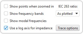
The control panel for the All SPL graph has these controls:

If Show points when zoomed in is selected the individual points
that make up the SPL and phase responses are shown on the graph when the zoom
level is high enough for them to be distinguished (which may only be over part
of the plot)
If Show frequency bands is selected the audio frequency bands
are shown in a stripe above the graph. The bands are:
- Infrasound: below 20 Hz
- Sub bass: 20 to 60 Hz
- Bass: 60 to 250 Hz
- Low midrange: 250 to 500 Hz
- Midrange: 500 Hz to 2 kHz
- Upper midrange: 2 to 4 kHz
- Presence: 4 to 6 kHz
- Brilliance: 6 to 20 kHz
If Show modal frequencies is selected the theoretical modal
frequencies for the room dimensions entered in the
Modal Analysis section of the
EQ Window for the currently selected measurement are plotted at the bottom of the graph.
When impedance is being plotted the axis has a span from 0 to 1 kohm. If
a larger impedance range is required the axis can be switched to logarithmic
with a range up to 1 Mohm using the Use a log axis for impedance
check box. If selected a log axis will be used wherever impedance is plotted.
The IEC 263 ratio control allows the graph to be
locked to a specified dB/decade aspect ratio. The aspect ratio is maintained by
adjusting the margins around the graph as required.
The Trace options button brings up a dialog that allows the line
type of the graph traces to be changed.
